Monte Carlo Computer Simulation

The essence of computer simulation and its strength are easily explained by analogy: Suppose we want to know the average number of children in the American family. The only exact way to this knowledge is to ask each and every one of the eighty million or so mothers in the United States how many children they have, add the answers up, and divide by eighty million (or so).

Indeed. But unfortunately this is just the type of problem which has increasingly fallen into science's lap in this the waning twilight of the twentieth century. Such problems are often easy to state but impossible to solve, at least exactly. Aside from resigning ourselves to fin-de-siecle futilism, what's a body to do?

Well any reasonable person, confronted with the problem above, would suggest that we poll a representative sample of families -- say 20,000 -- and extrapolate the results. While the answer we get this way cannot by definition be exact, it would certainly be accurate enough for most purposes. And indeed polling is used to solve this type of problem daily, by pundits predicting political currents, advertisers gauging markets, producers gouging markets, and all of us in making our numerous daily judgments. (After all, the only way to be sure television is a wasteland is to watch it 24 hours a day, seven days a week. But most of us are comfortable issuing an opinion on the subject after a much shorter sampling.)

We can use the method of a representative poll to study complex physical systems, too -- systems such as a galaxy, the Earth's atmosphere, an advanced composite material, or the interior of a living cell. The problems that arise in studying these systems are not unlike the problem of determining the average size of the American family. Often the only way to calculate exactly the properties of these systems is to know the exact trajectory of each of the the billions of atoms that compose them. Such a calculation is well-defined and straightforward, but is clearly impossible practically.

What is often done these days is therefore to calculate the properties of interest for a representative sample (an ``ensemble'') of the allowed states of the system. The applet on the previous page allows you to do just this for a simple model of a flexible macromolecule.

Polling is big business, scientifically and otherwise, because when done correctly it allows one to predict approximately but accurately what is impossible to calculate exactly. It's worth remembering that their are two sources of error in every poll:

1. Statistical. If the sample isn't large enough, it won't reflect the whole. If we asked just two American mothers how many kids they had, we'd be on shaky grounds guessing that the answer for the entire United States is 40 million times this number. Statistical error is relatively easy to detect: you just increase the sample size a bit and see if the answers change. If they do, the sample was too small. When the answers are independent of the sample size the sample is big enough.

   There are also powerful mathematical techniques for estimating the size of the statistical error from the size of the sample. The statistical error which these methods predict is what is typically meant by the ``margin of accuracy'' pollsters claim for their polls.

2. Methodological. So how is it that polls can claim a ``margin of accuracy'' of ±3% and then predict something screwy like Dewey beats Truman? Because errors in the method of polling sometimes occur, and these are generally more important than any statistical error. If, for example, we polled only Asian families or poor families, our results for the average size of the American family would be grossly incorrect no matter how large our sample was.

   Unlike statistical errors, methodological errors are generally hard to uncover and impossible to estimate, because there is no reliable test for their presence and magnitude, and they can often be fiendishly subtle.

Here are several important classes of polymers which may be familiar:

Plastics. Yep, the dude in The Graduate was right -- plastics are a huge business. Ordinary plastic materials such as are found in soda bottles, milk jugs, sewer pipes, clothing, rugs, cars, eyeglasses, plastic and rubber tubing, etc. are a multibillion dollar industry. Furthermore, nearly all of the ``advanced'' materials that one hopes will lead to such miracles as, say, a lining for an artificial heart that does not produce deadly blood clots, or a car light enough to be powered entirely by solar cells, are polymeric. From printed circuit boards to compact discs industrial polymers utterly dominate our technological materials landscape.

DNA and RNA. The old double helix of life itself -- a polymer. The longest known polymer, in fact, since it can reach several inches in length in higher mammals and become easily visible under an ordinary light microscope when properly prepared. The endless patterns in which one can rearrange the four types of railroad cars making up this train are the source of the variety of life.

Proteins. The main constituent of living cells, proteins are polymers with twenty different types of cars in the train -- the twenty amino acids. Some proteins such as silk and wool could be considered industrial products, since they see a great deal of commercial use in fabrics.

Polysaccharides. Made from the coupling of sugar molecules. A familiar form is cellulose, the main ingredient of cotton and rayon. Other forms include pectin, the material most commonly used to make jellies and jams, and chitin, the material of which the tough exoskeletons of insects is made.

Suppose we imagine a very simple model of a polymer:

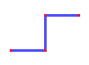
So how many states (shapes) are possible for this model polymer? If we had only four monomers, there would be just two possibilities:

R =

R1 + R2 ------ 2

=

1 + 5 ------ 2

= 1.618

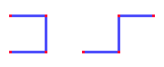
Cool. Now what if we have a bigger molecule? If we have 5 atoms we have 4 possible shapes,

R =

R1 + R2 + R3 + R4 ------------- 4

=

8 + 2 + 2 + 0 --------- 4

= 1.707

For 8 atoms we have these 32 possible shapes,

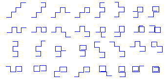
and we could (with effort) calculate R exactly once again. But for 12 atoms we have 512 shapes, for 20 atoms 131,072 shapes, for 25 atoms 4 million shapes, for 30 atoms a billion shapes, and for a mere 275 atoms more shapes (about 10⁸²) then there are atoms in the observable universe.

We must conclude that for any serious polymer (which typically has between 100 and 10,000 units) we are not going to be able to calculate its average size exactly by sitting down and figuring out each possible shape and its size.

The applet on the previous page puts you at the controls of a very commonly used method of constructing a representative ensemble: Monte-Carlo computer simulation with Metropolis importance sampling. (``Metropolis'' is somebody's name -- it has nothing to do with Superman's home.) If you manipulate the controls you can generate a representative ensemble of shapes (``conformations'') of a model polymer similar to the model discussed above. As you generate the members of the ensemble, the applet will keep track of their squared end-to-end distance R². You can command the applet to calculate the average value of this quantity < R² > and even the complete probability distribution P(R²) of R². The quantity P(R²) is just the probability that if you take a look at the polymer it will have a squared end-to-end distance equal to R². Another way of looking at this is that, if one has a very large number of polymers, P(R²) is proportional to how many of them will have squared end-to-end distance equal to R².

The model of the polymer used in the applet is very similar to the model discussed above. One further simplication has been made: neighboring bonds between monomers are allowed to be at angles of 0° and 180° with respect to one another as well as 90°. The reason for this simplification is, as will be explained later, this allows one to calculate the properties of the polymer exactly by statistical mechanics, for comparison to the results of the computer simulation.

An optional additional complication has been added: one can turn on an electric field pointing straight up. We imagine that each bond of the polymer has an electric dipole moment (real bonds in polymers often do), which will want to align with the electric field. When the field is turned on, the energy of any polymer shape is given by the number of bonds pointed oppositely from the field (down) minus the number of bonds pointed along the field (up), times the electric field strength. Thus different shapes of the polymer have slightly different energies. As you would guess, this means they have different probabilities of occuring.

Most recently added member.

The big picture shows you the shape that was added most recently to the ensemble.

Control panel.

At the top of the simulation you will see a control panel showing the number of monomers in the chain N, the electric field strength E, the temperature T, and the present size of the ensemble (``#''). You will also see the energy and squared end-to-end distance ``R^2'' of the most recently added ensemble member (shown in the big picture).

Zoom in/out buttons.

The buttons labeled ``+'' and ``-'' will zoom the big picture in and out.

step button.

If you press the button labeled ``step'' the applet will try to generate a new member of the ensemble. If it succeeds you will see the new member in the big picture, and the control panel will be updated.

go/stop button.

If you press the button labeled ``go'' the applet will continuously generate new members of the ensemble as fast as it can. Press the button again to stop this madness.

RESET button.

To discard your ensemble and start all over, press the ``RESET'' button. To begin with a different number of monomers in the chain, type the number of monomers you want into the window next to the ``N = '' label, and then press the RESET button.

E and T sliders.

Control the electric field strength E and temperature T with the two sliders at the left side of the big picture. Your changes take effect immediately -- you don't need to press the RESET button.

P(R^2) on/off.

If you press this button, you will toggle the display of the squared end-to-end distance averaged over all present members of the ensemble, as well as the present probability distribution of R^2. The display will appear in a seperate window. To close this window, press the ``P(R^2) off'' button. The average and P(R^2) are updated each time the ensemble grows whether or not this display is visible.

detail on/off.

Pressing this button will toggle the display of the details of the Metropolis algorithm for selecting new members of the ensemble. You will see the change in energy each proposed new member would create, the Boltzmann factor (see below) this involves, and the random number generated to decide whether or not to accept the trial member. You will also see whether the trial member was accepted (``ADDED'') or not (``REJECTED''), how many trial members have been considered so far (``tries'') and what percentage were accepted (``0K''). Furthermore, while this window is open the big picture will display each trial member that is rejected in light color, superimposed on the last accepted member.

To return to the starting situation, if the applet gets confused, you can try pressing the Reload button on your browser while holding down the Shift key at the same time. If the applet does truly strange things, though, please contact the author so he can try to fix them.

If the electric field strength is not zero, then some shapes have higher energy than others and, as one would expect, the polymer is less likely to be found in shapes of higher energy. The exact probability of the polymer being in a given shape of energy E is given by the Boltzmann factor

P(E) = Z ^-1 e ^{- E / k T}

where Z and k are constants and T is the temperature. (This means the ensemble constructed here is the so-called ``canonical ensemble''. For more information on the canonical ensemble and a simple derivation of the Boltzmann factor, visit the Ideal Atmosphere applet.)

To generate members of the ensemble in such a way that the probability of a given conformation appearing in the ensemble is equal to its Boltzmann factor, we use the Metropolis algorithm, as follows:

1. We generate a new ``trial'' conformation and calculate its energy E_new.

2. If E_new is less than the energy of the conformation we last added to the ensemble (call this E_old), then we accept the trial member into the ensemble.

3. If E_new > E_old, we perform the following test: We calculate the Boltzmann factor for the increase in energy:

   B = e ^{- (E_new - E_old) / k T}

   and then we compare this factor to a random number x between 0.0 and 1.0. If B > x, we accept the trial conformation, otherwise we reject it.